L'animation
import numpy as np
from matplotlib import pyplot as plt
from matplotlib import animation
import math
from IPython.display import HTML

# First set up the figure, the axis, and the plot element we want to animate
fig = plt.figure()

ax = plt.axes(xlim=(-5, 15), ylim=(-5, 20))
ax.grid()
ax.axhline(0)
ax.axvline(0)
line, = ax.plot([], [], lw=2)
anglemax = math.atan(6/5)
nbframe = 200
cursor = anglemax/nbframe

time_point, = ax.plot([], [], marker='o', markersize = '8')
rect, = ax.plot([0,10,10,0,0], [0,0,6,6,0], 'r-', lw = 4 )
time_line, = ax.plot([], [], 'b-', lw = 4)
time_text = ax.text(3, 12, '', fontsize = 12)
time_template = r"($\alpha$, $g(\alpha) = \frac{10}{\cos \alpha} + 6 - 5 \frac{\sin \alpha}{\cos \alpha}$) =( %1.2f, %1.2f )"

def g(t):
    return 10 / math.cos(t) + 6 - 5 * math.tan(t)

# initialization function: plot the background of each frame
def init():
    time_line.set_data([], [])
    time_point.set_data([], [])
    time_text.set_text('')
    return time_line, time_point, time_text

# animation function.  This is called sequentially
def animate(i):
    alpha = i*cursor
    h = 6 - 5 * math.tan(alpha)
    L = g(alpha)
    x = [0,5,10,5,5]
    y = [6,h,6,h,0]
    time_line.set_data(x, y)
    time_point.set_data([alpha], [L])
    time_text.set_text(time_template % (alpha, L) )
    return time_line, time_point, time_text

# call the animator.  blit=True means only re-draw the parts that have changed.
anim = animation.FuncAnimation(fig, animate, init_func=init,
                               frames=200, interval=20, blit=True)


# save the animation as an mp4.  This requires ffmpeg or mencoder to be
# installed.  The extra_args ensure that the x264 codec is used, so that
# the video can be embedded in html5.  You may need to adjust this for
# your system: for more information, see
# http://matplotlib.sourceforge.net/api/animation_api.html
# anim.save('TP4_animation.mp4', fps=30, extra_args=['-vcodec', 'libx264', '-pix_fmt', 'yuv420p'])

HTML(anim.to_html5_video())
La solution mathématique
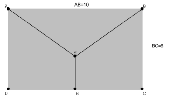
Longueur totale de la conduite : $MA + MB + MH$.
On considère le point $Q$, projeté orthogonal de $M$ sur $BC$ et on note $\alpha$ l'angle $\widehat{QMB}$.
On a $\alpha \in [0 ; S [$ avec $S < \frac{\pi}{2}$ . En fait on a $S = \tan^{-1}(\frac{6}{5})$).
Dans le triangle $QMB$ rectangle en $M$ on a $ \cos \alpha = \frac{QM}{MB} = \frac{5}{MB} \Leftrightarrow MB = \frac{5}{\cos \alpha}$.
Par symétrie axiale d'axe la médiatrice de $[AB]$ on a $MA=MB$.
Dans le triangle $QMB$ rectangle en $M$ on a $ \sin \alpha = \frac{QB}{MB} = \frac{QB \cos \alpha}{5} \Leftrightarrow QB = 5\frac{\sin \alpha}{\cos \alpha}$.
De plus on a $MH = 6 - QB = 6 - \frac{5 \sin \alpha}{\cos \alpha}$
On en déduit que la longueur de la conduite est $g(\alpha)=2 \times \frac{5}{\cos \alpha} + 6 - 5\frac{\sin \alpha}{\cos \alpha}$.
Calculons la dérivée de la fonction g
from sympy import *
init_session()
def deriver(f, x):
    return simplify(diff(f, x))
g = 10 / cos(x) + 6 - 5 * sin(x) / cos(x)
deriver(g, x)
Etudions le signe de la dérivée de $g$
Pour tout réel $\alpha \in [0 ; S [$ avec $S < \frac{\pi}{2}$ on a $\cos^{2} \alpha > 0$ donc $g'(\alpha)$ est du signe de $10 \sin \alpha - 5$.
Sur l'intervalle $[0 ; S [$ avec $S < \frac{\pi}{2}$ on a : $$ 10 \sin \alpha - 5 = 0 \Leftrightarrow \sin \alpha = \frac{1}{2} $$ $$ 10 \sin \alpha - 5 = 0 \Leftrightarrow \alpha = \frac{\pi}{6} $$ et $$ 10 \sin \alpha - 5 > 0 \Leftrightarrow \sin \alpha > \frac{1}{2} $$ $$ 10 \sin \alpha - 5 > 0 \Leftrightarrow \alpha > \frac{\pi}{6} $$ et $$ 10 \sin \alpha - 5 < 0 \Leftrightarrow \sin \alpha < \frac{1}{2} $$ $$ 10 \sin \alpha - 5 < 0 \Leftrightarrow \alpha < \frac{\pi}{6} $$
On en déduit que $g$ est strictement décroissante sur $[0; \frac{\pi}{6}]$ et strictement croissante sur $ [\frac{\pi}{6} ; S [$ avec $S < \frac{\pi}{2}$. La longueur de la conduite est donc minimale pour $\alpha = \frac{\pi}{6}$.